WELCOME TO INDEX TO CRAIN'S PERSONAL AMD RAILROAD PAGES
Home Page / Index | Search
Personal Stuff • Petrophysicist, Educator, Entrepreneur, Rancher - My Resume • Travels in Purgatory - Memoir of an Itinerant Petrophysicist
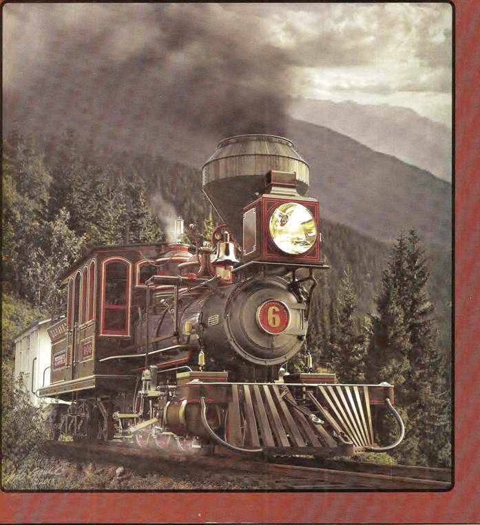
• Crain's Petrophysical Handbook - Online HERE • Free Publications • Project List • Client List • A Small Piece of Paradise - My Ranching Story The South Park Line (DSP&P RR) • General Interest Articles • Rolling Stock Histories, Photos, Plans, Rosters • Rolling Stock Plan Collections • Rolling Stock Plans by Specialists • Rolling Stock Specifications
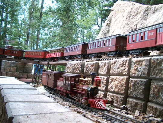
My Model Trains • My South Park Line in the Garden - Story and Photo Galleries • Dressing Up Large Scale Models - More Realism • My South Park Photo Roster - Large Format Images of Large Scale Models • FOR SALE From My South Park Collection - Rare and Unique Large Scale • My Rocky Mountain Railway in the Garage - Malcolm Furlow's "LGB Empire" • 70 Years - 7 Model Railways - and the Men Who Inspired Them • Large Scale Basics - Scales, Wiring, Scenery, Sound, Much More
• Scale / Gauge Encyclopedia - Definitions, Standards, Info Tables
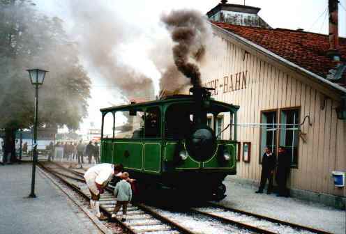
Vintage Train Travels • "The Canadian", "The Rocky Mountaineer", and Other Gems • Colorado Narrow Gauge Circle • California Nevada Circle • Germany, Austria, Switzerland • Fiji, Australia, China, Hong Kong • Railroad Museums and Heritage Parks Mini World Atlas • Africa and Indian Ocean • Asia and Middle East • Australia and Pacific Ocean • Europe and North Atlantic • North and South America, Caribbean
Copyright © 2022 E. R. (Ross) Crain, P.Eng. email